Formulas & Functions Excel 2007 - 13. Analyzing Data with Tables (1 người xem)

[BNTT]

Phỏng dịch từ cuốn Formulas and Functions with Microsoft Office Excel 2007 của Paul McFedries

Phần III: Xây dựng các mô hình kinh doanh

• Chương 13: Phân tích dữ liệu với các Table
  
  
• Chương 14: Phân tích dữ liệu với các PivotTable
  
  
• Chương 15: Sử dụng các công cụ tạo mô hình kinh doanh của Excel

---------------------------------------------------------------------------------------


PART III - BUILDING BUSINESS MODELS
Phần III - Xây dựng các mô hình kinh doanh


Chapter 13 - ANALYZING DATA WITH TABLES
Chương 13 - Phân tích dữ liệu với các Table

Excel’s forte is spreadsheet work, of course, but its row-and-column layout also makes it a natural flat-file database manager. In Excel, a table is a collection of related information with an organizational structure that makes it easy to find or extract data from its contents. (In previous versions of Excel, a table was called a list.) Specifically, a table is a worksheet range that has the following properties:
Dĩ nhiên rằng, sở trường của Excel là làm việc với các bảng tính, nhưng các bố cục hàng và cột của nó cũng làm cho nó trở thành một trình quản lý cơ sở dữ liệu phẳng. Trong Excel, một Table là một tập hợp thông tin liên quan, cấu trúc có tổ chức, nhằm giúp dễ dàng tìm kiếm hoặc trích xuất dữ liệu nội dung của nó. (Trong các phiên bản trước của Excel, một Table được gọi là một List.) Cụ thể, một Table là một dãy bảng tính có những đặc điểm sau đây:

• Field — A single type of information, such as a name, an address, or a phone number. In Excel tables, each column is a field.
  Một loại thông tin như là tên, địa chỉ, số điện thoại... Trong Excel, mỗi cột là một Field.
  
  
• Field value — A single item in a field. In an Excel table, the field values are the individual cells.
  Một mục đơn trong một field. Trong một Table của Excel, các Field Value là các ô đơn lẻ.
  
  
• Field name — A unique name you assign to every table field (worksheet column). These names are always found in the first row of the table.
  Một tên duy nhất mà bạn gán cho mỗi Field của Table (cột trong bảng tính). Những tên này luôn luôn được tìm thấy trong hàng đầu tiên của Table.
  
  
• Record — A collection of associated field values. In Excel tables, each row is a record.
  Một tập hợp kết hợp các Field Value. Trong Table của Excel, mỗi hàng là một Record.
  
  
• Table range — The worksheet range that includes all the records, fields, and field names of a table.
  Một vùng bảng tính bao gồm tất cả các Record, Field, và Field Name của một Table.

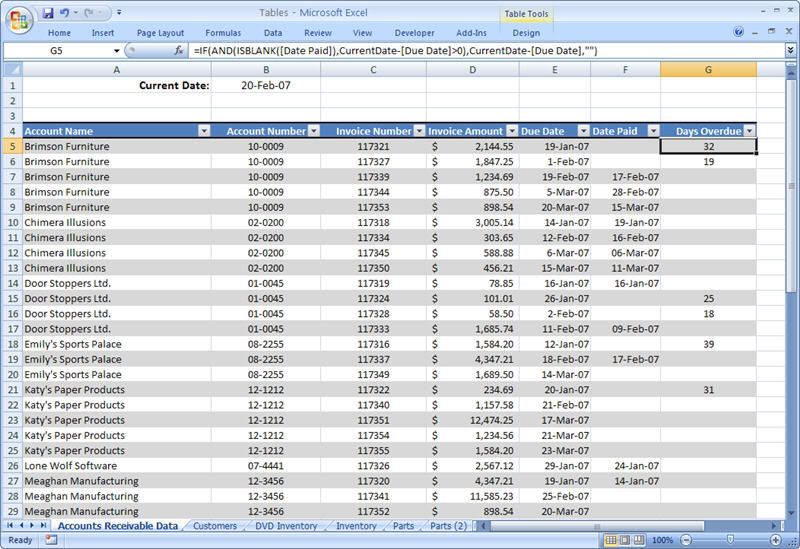
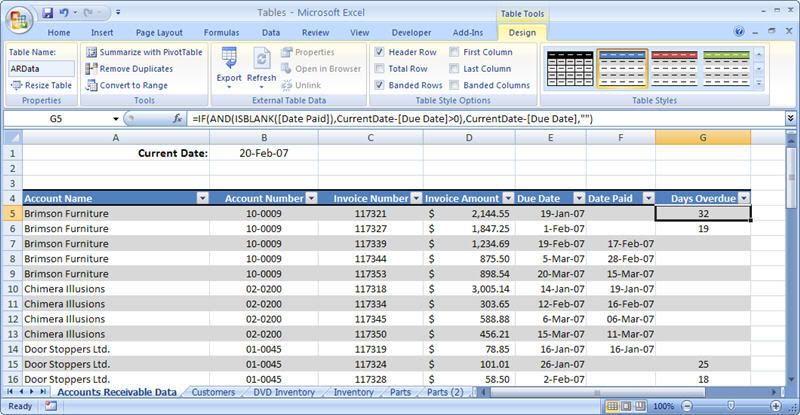
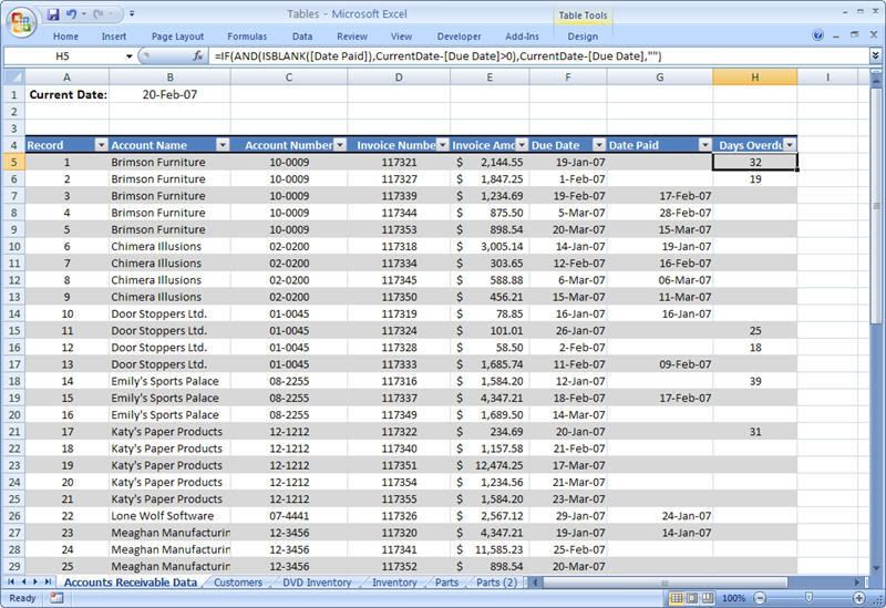
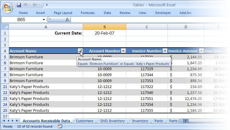
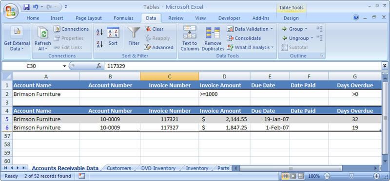
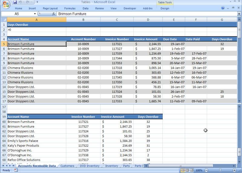
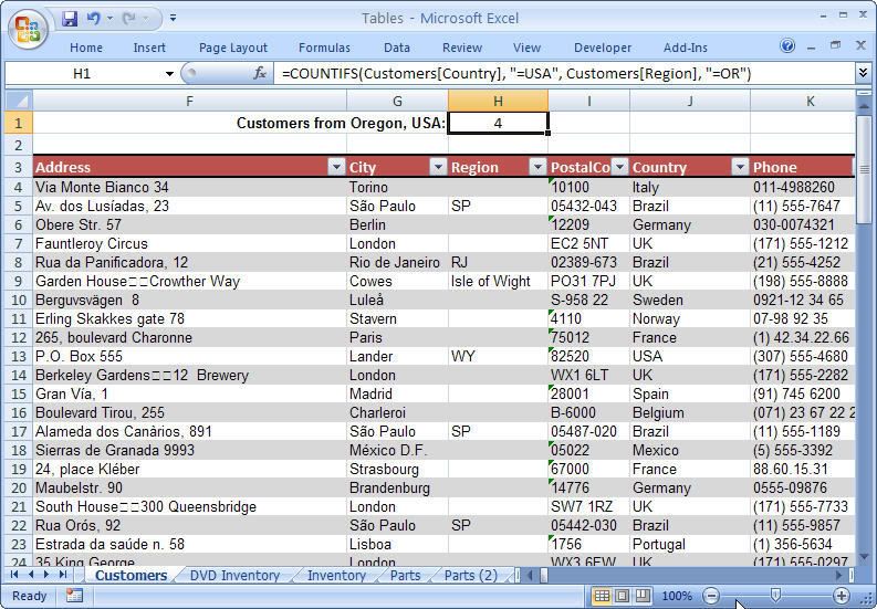
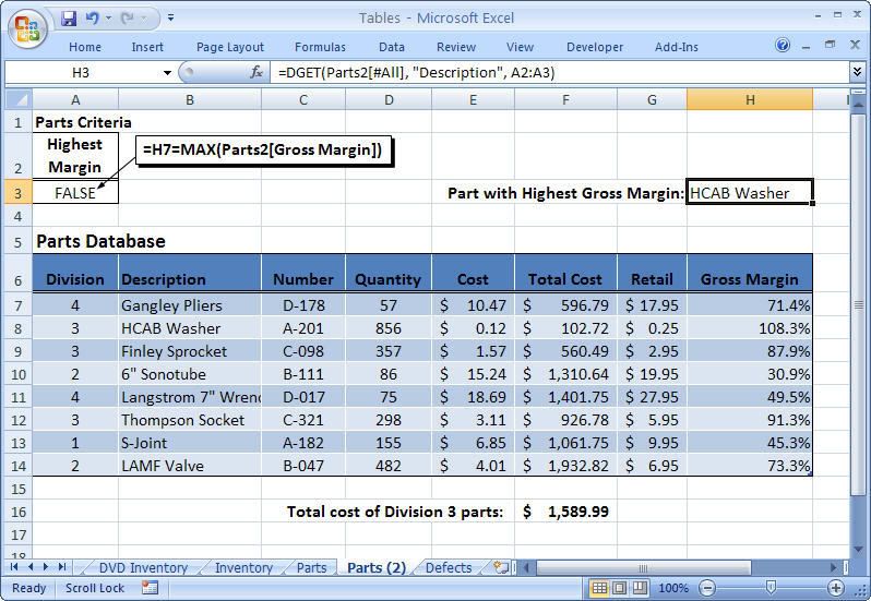
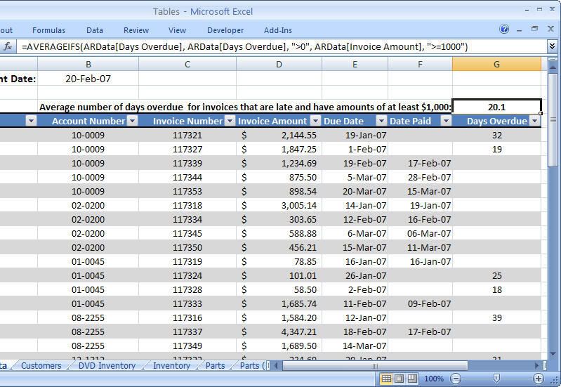
For example, suppose that you want to set up an accounts receivable table. A simple system would include information such as the account name, account number, invoice number, invoice amount, due date, and date paid, as well as a calculation of the number of days overdue. Figure 13.1 shows how this system would be implemented as an Excel table.
Ví dụ, giả sử rằng bạn muốn thiết lập một bảng gồm các khoản phải thu. Một hệ thống đơn giản thường bao gồm những thông tin như tên tài khoản, mã tài khoản, số hóa đơn, giá trị hóa đơn, thời hạn thanh toán, ngày thanh toán, cũng như những phép tính số ngày quá hạn. Hình 13.1 minh họa một hệ thống như vậy sẽ được thực thi dưới dạng Table của Excel như thế nào.

Figure 13.1 - Tables.xlsx​

Excel tables don’t require elaborate planning, but you should follow a few guidelines for best results. Here are some pointers:
Table của Excel không yêu cầu phải lên một kế hoạch chi tiết, nhưng bạn nên theo những hướng dẫn sau đây để có được kết quả tốt nhất. Đây là một số điểm chính:

• Always use the top row of the table for the column labels.
  Luôn luôn dùng hàng trên cùng của Table để làm các tiêu đề cột.
  
  
• Field names must be unique, and they must be text or text formulas. If you need to use numbers, format them as text.
  Các Field Name phải là duy nhất, và chúng phải là text hoặc là công thức ở dạng text. Nếu bạn cần dùng các con số, hãy định dạng chúng thành dạng text.
  
  
• Some Excel commands can automatically identify the size and shape of a table. To avoid confusing such commands, try to use only one table per worksheet. If you have multiple related tables, include them in other worksheets in the same workbook.
  Một số lệnh trong Excel có thể làm cho kích thước và hình dạng của một Table tự động điều chỉnh. Để tránh nhầm lẫn những lệnh như vậy, bạn cố gắng chỉ sử dụng một Table trong một trang tính (worksheet). Nếu bạn có nhiều Table liên quan với nhau, bạn hãy để chúng trong từng trang tính của cùng một bảng tính (workbook).
  
  
• If you have nonlist data in the same worksheet, leave at least one blank row or column between the data and the table. This helps Excel to identify the table automatically.
  Nếu bạn có một dữ liệu mà không phải là một Table trong cùng một trang tính, hãy chừa ra ít nhất một hàng trống hoặc một cột trống giữa dữ liệu của bạn với Table. Điều này giúp cho Excel dễ dàng tự động nhận ra một Table.
  
  
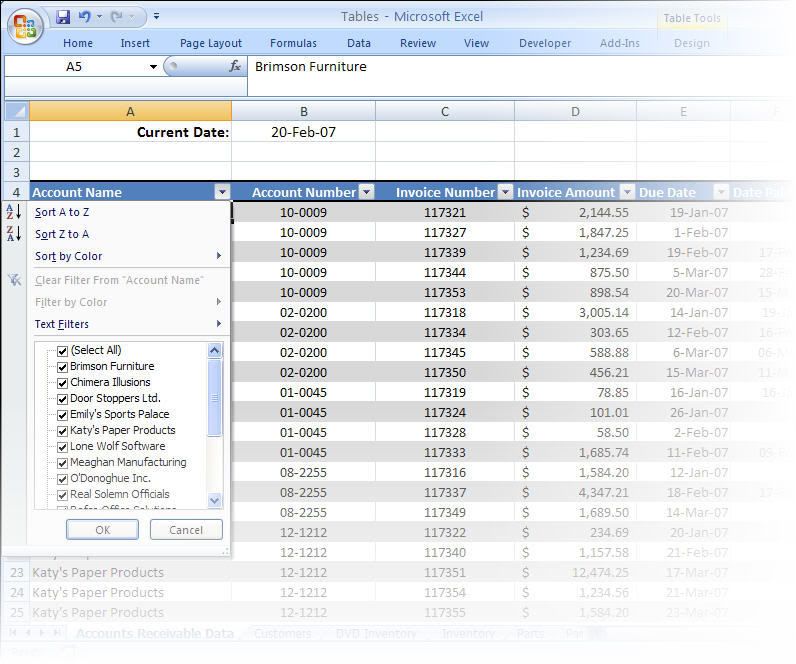
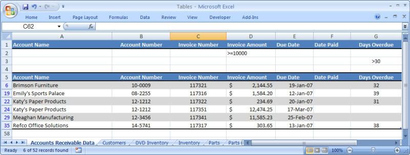
• Excel has a command that enables you to filter your table data to show only records that match certain criteria. (See “Filtering Table Data,” later in this chapter, for details.) This command works by hiding rows of data. Therefore, if the same worksheet contains nonlist data that you need to see or work with, don’t place this data to the left or right of the table.
  Excel có một lệnh cho phép bạn lọc dữ liệu trong Table để chỉ thấy những Record theo những tiêu chuẩn nhất định (xem phần “Lọc dữ liệu trong Table”, ở phần sau của chương này, để biết thêm chi tiết). Lệnh này làm việc bẳng cách ẩn đi một số hàng trong dữ liệu. Do đó, nếu trong cùng một trang tính mà có chứa một dữ liệu thường và bạn cần phải thấy được để làm làm việc với nó, bạn đừng đặt dữ liệu này ở bên phải hay bên trái của Table.

You can download the workbook that contains this chapter’s examples here:
Bạn có thể tải về bảng tính với những ví dụ trong chương này tại đây: Example Files

 

[BNTT]

Chapter 13 - Analyzing Data with Tables


13.1. Converting a Range to a Table
Chuyển đổi một dãy thành một Table

Excel has a number of commands that enable you to work efficiently with table data. To take advantage of these commands, you must convert your data from a normal range to a table. Here are the steps to follow:
Excel có một số lệnh cho phép bạn làm việc hiệu quả với Table dữ liệu. Để tận dụng những lệnh này, bạn phải chuyển đổi dữ liệu của bạn từ một dãy bình thường thành một Table. Đây là các bước để theo:

1. Click any cell within the range that you want to convert to a table.
   Nhấp vào bất kỳ ô nào trong dãy mà bạn muốn chuyển đổi thành một Table.
   
   
2. You now have two choices:
   Bạn có hai lựa chọn:
   
   
   • To create a table with the default formatting, choose Insert, Table (or press Ctrl+T).
     Để tạo một Table với những định dạng mặc định, bạn chọn Insert, Table (hoặc nhấn Ctrl+T).
     
     
   • To create a table with the formatting you specify, choose Home, Format as Table, and then click a table style in the gallery that appears.
     Để tạo một Table với những định dạng do bạn chỉ định, bạn chọn Home, Format as Table, và rồi nhấn vào một kiểu Table trong thư viện.
   
   
   
3. Excel displays the Create Table dialog box. The Where Is the Data for Your Table? box should already show the correct range coordinates. If not, enter the range co-ordinates or select the range directly on the worksheet.
   Excel hiển thị hộp thoại Create Table. Thường thì hộp Where Is the Data for Your Table? đã trình bày sẵn tọa độ chính xác. Nếu không, bạn nhập tọa độ dãy vào hoặc chọn trực tiếp dãy trên trang tính.
   
   
4. If your range has column headers in the top row (as it should), make sure the My Table Has Headers check box is activated.
   Nếu dãy của bạn có các tiêu đề cột trên hàng trên dùng (thường là có), hãy chắc chắn rằng hộp kiểm My Table Has Headers được kích hoạt.
   
   
5. Click OK.
   Nhấn OK.

When you convert a range to a table, Excel makes three changes to the range, as shown in Figure 13.2:
Khi bạn chuyển đổi một dãy thành một Table, Excel sẽ thay đổi ba thứ sau trong dãy, như minh họa ở hình 13.2:

• It formats the table cells.
  Nó định dạng các ô trong Table.
  
  
• It adds drop-down arrows to each field header.
  Nó thêm các mũi tên drop-down (như khi bạn chọn AutoFilter) vào mỗi tiêu đề Field.
  
  
• In the Ribbon, you see a new Design tab under Table Tools whenever you select a cell within the table.
  Trên thanh Ribbon, bạn thấy có thêm một tab Design nằm bên dưới Table Tools mỗi khi bạn chọn bất kỳ một ô nào trong Table.

Figure 13.2 - Tables.xlsx​

If you ever need to change the table back to a range, select a cell within the table and choose Design, Convert to Range.
Nếu bạn lại muốn chuyển đổi Table trở lại thành một dãy bình thường, bạn chọn một ô bất kỳ trong Table, rồi chọn Design, Convert to Range.​

 

[BNTT]

Chapter 13 - Analyzing Data with Tables


13.2. Basic Table Operations
Các thao tác cơ bản với Table

After you’ve converted the range to a table, you can start working with the data. Here’s a quick look at some basic table operations:
Sau khi bạn đã chuyển đổi dãy thành một Table, bạn có thể bắt đầu làm việc với dữ liệu. Sau đây là sơ lược một vài thao tác cơ bản với Table:

• Selecting a record — Move the mouse pointer to the left edge of the leftmost column in the row you want to select (the pointer changes to a right-pointing arrow) and then click. You can also select any cell in the record and then press Shift+Space.
  Chọn một Record (một hàng trong Table) — Di chuyển con trỏ chuột sang mép phải của cột cuối cùng bên trái trong hàng mà bạn muốn chọn (con trỏ sẽ đổi thành một mũi tên hướng sang phải) và nhấn chuột. Bạn cũng có thể chọn bất kỳ ô nào trong Record rồi nhấn Shift+Space.
  
  
• Selecting a field — Move the mouse pointer to the top edge of the column header (the pointer changes to a downward-pointing arrow). Click once to select just the field’s data; click a second time to add the field’s header to the selection. You can also select any cell in the field and then press Ctrl+Space to select the field data; press Ctrl+Space again to add the header to the selection.
  Chọn một Field (một cột trong Table) — Di chuyển con trỏ chuột đến mép trên cùng của tiêu đề cột (con trỏ sẽ đổi thành một mũi tên hướng xuống). Nhấn một cái để chỉ chọn dữ liệu của Field; nhấn thêm một lần nữa để thêm tiêu đề của Field vào vùng chọn. Bạn cũng có thể chọn bất kỳ ô nào trong Field rồi nhấn Ctrl+Space để chọn dữ liệu của Field, nhấn Ctrl+Space thêm một lần nữa để thêm tiêu đề của Field vào vùng chọn.
  
  
• Selecting the entire table — Move the mouse pointer to the upper-left corner of the table (the pointer changes to an arrow pointing down and to the right) and then click. You can also select any cell in the table and press Ctrl+A.
  Chọn toàn bộ Table — Di chuyển con trỏ chuột đến góc trên cùng bên trái của Table (con trỏ sẽ đổi thành một mũi tên hướng xuống và nghiêng sang phải) rồi nhấn chuột. Bạn cũng có thể chọn bất kỳ ô nào trong Table rồi nhấn Ctrl+A.
  
  
• Adding a new record at the bottom of the table — Select any cell in the row below the table, type the data you want to add to the cell, and press Enter. Excel 2007’s new AutoExpansion feature expands the table to include the new row. This also works if you select the last cell in the last row of the table and then press Tab.
  Thêm một Record (hàng) mới vào cuối một Table — Chọn bất kỳ ô nào ở một hàng ngay sát bên dưới Table, nhập dữ liệu vào mà bạn muốn thêm vào ô, và nhấn Enter. Chức năng AutoExpansion của Excel 2007 tự động mở rộng Table để chứa thêm hàng mới. Nó cũng tự động thêm một hàng mới vào nếu bạn đứng ở ô cuối cùng trong hàng cuối cùng của Table mà nhấn phím Tab.
  
  
• Adding a new record anywhere in the table — Select any cell in a record below which you want to add the new record. In the Home tab, choose Insert, Insert Table Rows Above. Excel inserts a blank row above the selected cell into which you can enter the new data.
  Thêm một Record (hàng) mới vào bất kỳ nơi nào trong Table — Chọn bất kỳ ô nào trong một hàng ở dưới cái hàng mà bạn muốn thêm một hàng mới vào. Trong tab Home, chọn Insert, Insert Table Rows Above (để nhanh hơn, bạn có thể dùng Shortcut menu với phím phải chuột, trong đó cũng có lệnh này). Excel sẽ thêm một hàng mới vào ở trên ô đang chọn để bạn nhập thêm dữ liệu mới.
  
  
• Adding a new field to the right of the table — Select any cell in the column to the right of the table, type the data you want to add to the cell, and press Enter. AutoExpansion expands the table to include the new field.
  Thêm một Field (cột) mới vào bên phải của Table — Chọn bất kỳ ô nào ở cột ngay sát bên phải của Table, nhập dữ liệu vào mà bạn muốn thêm vào ô, và nhấn Enter. Chức năng AutoExpansion của Excel 2007 tự động mở rộng Table để chứa thêm Field mới.
  
  
• Adding a new field anywhere in the table — Select any cell in a column to the right of which you want to add the new field. In the Home tab, choose Insert, Insert Table Columns to the Left. Excel inserts a blank field to the left of the selected cell.
  Thêm một Field (cột) mới vào bất kỳ nơi nào trong Table — Chọn bất kỳ ô nào trong một cột ở bên phải cái cột mà bạn muốn thêm một cột mới vào. Trong tab Home, chọn Insert, nsert Table Columns to the Left (để nhanh hơn, bạn có thể dùng Shortcut menu với phím phải chuột, trong đó cũng có lệnh này). Excel sẽ thêm một cột mới vào ở bên trái ô đang chọn.
  
  
• Deleting a record — Select any cell in the record you want to delete. In the Home tab, choose Delete, Delete Table Rows.
  Xóa một Record (hàng) — Chọn bất kỳ ô nào trong hàng mà bạn muốn xóa. Trong Home tab, chọn Delete, Delete Table Rows (cũng có thể dùng Shortcut menu với phím phải chuột).
  
  
• Deleting a field — Select any cell in the field you want to delete. In the Home tab, choose Delete, Delete Table Columns.
  Xóa một Field (cột) — Chọn bất kỳ ô nào trong cột mà bạn muốn xóa. Trong Home tab, chọn Delete, Delete Table Columns (cũng có thể dùng Shortcut menu với phím phải chuột).
  
  
• Displaying Table Totals — If you want to see totals for one or more fields, click inside the table, choose the Design tab, and then click to activate the Total Row check box. Excel adds a Total row at the bottom of the table. Each cell in the Total row has a drop-down list that enables you to choose the function you want to use: Sum, Average, Count, Max, Min, and more.
  Hiển thị các thống kê của Table — Nếu bạn muốn xem những thống kê cho một hoặc nhiều Field, bạn nhấn vào bên trong Table, chọn tab Design, rồi kích hoạt hộp kiểm Total Row. Excel thêm một dòng Total vào dưới cùng của Table. Mỗi ô trong dòng Total này có một danh sách drop-down, cho phép bạn chọn hàm mà bạn muốn dùng: Sum, Average, Count, Max, Min, v.v...
  
  
• Formatting the table — Excel comes with a number of built-in table styles that you can apply with just a few mouse clicks. Click inside the table, choose the Design tab, and then choose a format in the Table Styles gallery. You can also use the check boxes in the Table Style Options group to toggle various table options, including Banded Rows and Banded Columns.
  Định dạng Table — Excel có một số mẫu định dạng Table mà bạn có thể áp dụng với vài cái nhấn chuột. Nhấn vào bên trong Table, chọn tab Design, rồi chọn một kiểu định dạng trong thư viện Table Styles. Bạn cũng có thể sử dụng những hộp kiểm trong nhóm Table Style Options để thêm bớt những tùy chọn định dạng, bao gồm cả Banded Rows và Banded Columns.
  
  
• Resizing the table — Resizing the table means adjusting the position of the lower-right corner of the table: move the corner down to add records; move the corner right to add fields; move the corner up to remove records from the table (the data remains intact, however); move the corner left to remove fields from the table (again, the data remains intact). The easiest way to do this is to click-and-drag the resize handle that appears in the table’s lower-right cell. You can also click inside the table and then click Design, Resize Table.
  Định lại kích thước Table — Định lại kích thước Table có nghĩa là điều chỉnh vị trí của ô nằm ở góc dưới cùng bên phải của Table: di chuyển ô này xuống để thêm Record (hàng); di chuyển sang phải để thêm Field (cột); di chuyển lên trên để bỏ bớt Record (nhưng dữ liệu phải còn nguyên vẹn); di chuyển sang trái để bỏ bớt Field (nhưng dữ liệu cũng phải còn nguyên vẹn). Cách dễ nhất để làm việc này là nhấn và rê cái nút định cỡ (resize handle) xuất hiện ở ô dưới cùng bên phải của Table. Bạn cũng có thể nhấn vào bên trong bảng rồi nhấn Design, Resize Table.
  
  
• Renaming a table — You’ll see later on that Excel 2007 enables you to reference table elements directly. Most of the time these references include the table name, so you should consider giving your tables meaningful and unique names. To rename a table, click inside the table and then choose the Design tab. In the Properties group, edit the Table Name text box.
  Đổi tên một Table — Trong các bài sau, bạn sẽ thấy Excel 2007 cho phép bạn tham chiếu trực tiếp đến các phần tử trong Table. Phần lớn các lần tham chiếu có bao gồm tên của Table, do đó bạn nên đặt cho Table của bạn cái tên có ý nghĩa và duy nhất. Để đổi tên một Table, bạn nhấn vào bên trong Table và chọn tab Design, trong nhóm Properties, sửa lại Table Name.

 

[BNTT]

Chapter 13 - Analyzing Data with Tables


13.3. Sorting a Table
Sắp xếp một Table

One of the advantages of a table is that you can rearrange the records so that they’re sorted alphabetically or numerically. This feature enables you to view the data in order by customer name, account number, part number, or any other field. You even can sort on multiple fields, which would enable you, for example, to sort a client table by state and then by name within each state.
Một trong những lợi thế của một Table là bạn có thể sắp xếp lại các thông tin, cho nên chúng thường được sắp xếp thứ tự theo ABC hay theo số. Tính năng này cho phép bạn xem dữ liệu theo tên khách hàng, theo số tài khoản, theo từng phần, hay theo bất kỳ một Field nào. Thậm chí, bạn có thể sắp xếp theo nhiều Field, ví dụ như bạn có thể sắp xếp một bảng theo tên của từng trạng thái, rồi trong mỗi trạng thái đó lại sắp xếp theo từng cái tên.

For quick sorts on a single field, you have two choices to get started:
Để sắp xếp nhanh một Field đơn, bạn có thể lựa chọn một trong hai cách sau để bắt đầu:

• Click anywhere inside the field and then click the Data tab.
  Nhấn vào bất kỳ nơi nào trong Field và chọn tab Data.
  
  
• Pull down the field’s drop-down arrow.
  Nhấn nút mũi tên drop-down của Field.

For an ascending sort, click Sort A to Z (or Sort Smallest to Largest for a numeric field, or Sort Oldest to Newest for a date field); for a descending sort, click Sort Z to A (or Sort Largest to Smallest for a numeric field, or Sort Newest to Oldest for a date field).
Để sắp xếp theo thứ tự tăng dần, bạn chọn Sort A to Z (hoặc Sort Smallest to Largest cho các Field chứa số, hoặc Sort Oldest to Newest cho các Field chứa ngày tháng); còn để sắp xếp theo thứ tự giảm dần, bạn chọn Sort Z to A (hoặc Sort Largest to Smallest cho các Field chứa số, hoặc Sort Newest to Oldest cho các Field chứa ngày tháng).

NOTE:

How Excel sorts the table depends on the data. Here’s the order Excel uses in an ascending sort:
Excel sắp xếp Table như thế nào còn tùy thuộc vào loại dữ liệu. Sau đây là cách Excel sử dụng để sắp xếp theo thứ tự tăng dần:

• Numbers: Largest negative to largest positive
  Các số: Từ số âm lớn nhất đến số dương lớn nhất
  
  
• Text: Space ! “ # $ % & ‘ ( ) * + , - . / 0 through 9 (when formatted as text) : ; < = > ? @ A through Z (Excel ignores case) [ \ ] ^ _ ‘ {, } ~
  Các ký tự hoặc chữ (theo thứ tự sau): Space (khoảng trắng) ! “ # $ % & ‘ ( ) * + , - . / 0 cho đến 9 (khi định dạng theo kiểu text) : ; < = > ? @ A cho đến Z (Excel bỏ qua chữ thường, chữ hoa) [ \ ] ^ _ ‘ {, } ~
  
  
• Logical: FALSE before TRUE
  Giá trị Logical: FALSE rồi mới đến TRUE
  
  
• Error: All error values are equal
  Lỗi: Tất cả các lỗi đều như nhau
  
  
• Blank: Always sorted last (ascending or descending)
  Ô rỗng: Luôn luôn sắp xếp sau cùng (tăng dần cũng như giảm dần)

For more complex sorts on multiple fields, follow these steps:
Đối với những sắp xếp phức tạp hơn trong nhiều Field, bạn theo các bước sau:

1. Select a cell inside the table.
   Chọn một ô bên trong Table.
   
   
2. Choose Data, Sort. Excel displays the Sort dialog box, shown in Figure 13.3.
   Chọn Data, Sort. Excel hiển thị hộp thoại Sort như minh họa ở hình 13.3.
   
   
   

   
   Figure 13.3​
   
   
3. Use the Sort By list to click the field you want to use for the overall order for the sort.
   Dùng danh sách Sort By để chọn Field mà bạn muốn dùng để sắp xếp toàn bộ dữ liệu theo nó.
   
   
4. Use the Order list to select either an ascending or descending sort.
   Dùng danh sách Order để chọn một kiểu sắp xếp (tăng dần hay giảm dần)
   
   
5. (Optional) If you want to sort the data on more than one field, click Add Level, use the Then By list to click the field, and then select a sort order. Repeat for any other fields you want to include in the sort.
   (Tùy chọn) Nếu bạn muốn sắp xếp dữ liệu theo nhiều hơn một Field, bạn nhấn Add Level rồi chọn Field cho mục Then By, và rồi chọn cách sắp xếp. Lập lại bước này cho bất kỳ Field nào bạn muốn bao gồm trong việc sắp xếp này.
   

   NOTE:
   

   In previous versions of Excel, you could specify only a maximum of three sorting levels. In Excel 2007, you can specify up to 64 sorting levels.
   Trong những phiên bản trước của Excel, bạn chỉ có thể sắp xếp tối đa là theo 3 cấp độ. Trong Excel 2007, bạn có thể sắp theo đến 64 cấp độ.​

   
   

   CAUTION:
   

   Be careful when you sort table records that contain formulas. If the formulas use relative addresses that refer to cells outside their own record, the new sort order might change the references and produce erroneous results. If your table formulas must refer to cells outside the table, be sure to use absolute addresses.
   Hãy cẩn thận khi bạn sắp xếp những Record (hàng) có chứa công thức trong Table. Nếu các công thức dùng loại địa chỉ tương đối để tham chiếu đến những ô nằm ngoài Table, sự sắp xếp có thể làm thay đổi các tham chiếu và dẫn kết những kết quả sai. Nếu công thức trong Table của bạn có tham chiếu đến những ô ở ngoài Table, hãy chắc chắn bạn sử dụng loại địa chỉ tuyệt đối.​

   
   
6. (Optional) Click Options to specify one or more of the following sort controls:
   (Tùy chọn) Nhấn Option để xác định một hay nhiều kiểu sắp xếp sau:
   
   
   • Case Sensitive — Activate this check box to have Excel differentiate between uppercase and lowercase during sorting. In an ascending sort, for example, lowercase letters are sorted before uppercase letters.
     Kích hoạt hộp kiểm này để yêu cầu Excel phân biệt sự khác nhau giữa chữ thường và chữ hoa khi sắp xếp. Ví dụ, trong một sắp xếp tăng dần, những chữ thường luôn luôn được sắp xếp trước những chữ hoa.
     
     
   • Orientation — Excel normally sorts table rows (the Sort Top to Bottom option). To sort table columns, activate Sort Left to Right.
     Bình thường, Excel sắp xếp theo từng dòng (tùy chọn Sort Top to Bottom). Để sắp xếp theo cột, bạn kích hoạt mục Sort Left to Right.
   
   
7. Click OK. Excel sorts the table.
   Nhấn OK. Excel sắp xếp Table cho bạn.

 

[BNTT]

13.3. Sorting a Table


13.3.1. Sorting a Table in Natural Order
Sắp xếp một Table theo thứ tự lúc ban đầu

It’s often convenient to see the order in which records were entered into a table, or the natural order of the data. Normally, you can restore a table to its natural order by choosing Undo Sort in the Quick Access toolbar immediately after a sort.
Thứ tự khi nhập các record (hàng dữ liệu) vào trong một Table, hay thứ tự lúc ban đầu của dữ liệu, thì thường tiện lợi cho cách xem. Thông thường, bạn có thể phục hồi một Table trở về thứ tự lúc ban đầu của nó bằng lệnh Undo Sort trong thanh công cụ Quick Access sau khi thực hiện một sắp xếp.

Unfortunately, after several sort operations, it’s no longer possible to restore the natural order. The solution is to create a new field, for example, called Order, in which you assign consecutive numbers as you enter the data. The first record is 1, the second is 2, and so on. To restore the table to its natural order, you sort on the Order field.
Thật không may, sau vài thao tác sắp xếp, thì không còn có thể phục hồi lại thứ tự lúc ban đầu nữa. Giải pháp là, bạn tạo ra một field (cột) mới, ví dụ có tên là Record chẳng hạn, trong đó bạn gán các số liên tục vào khi bạn nhập liệu: Record (hàng) thứ nhất là 1, record thứ hai là 2, v.v... Để phục hồi lại Table theo thứ tự ban đầu của nó, bạn sắp xếp nó theo field Record này.

CAUTION:

The Record field only works if you add it either before you start inserting new records in the table, or before you’ve irrevocably sorted the table. Therefore, when planning any table, you might consider always including a Order field just in case you need it.
Field (cột) Record này chỉ làm việc khi bạn thêm nó vào trước khi bạn bắt đầu nhập các record (hàng) mới vào trong Table, hoặc là trước khi bạn sắp xếp Table lần đầu tiên. Bởi vậy, khi lập bất kỳ một Table nào, bạn nên luôn luôn thêm vào một field Record này, sẽ có những trường hợp bạn cần đến nó. ​

Follow these steps to add a new field to the table:
Theo những bước sau đây để thêm một field vào trong một Table:

1. Select a cell in the field to the right of where you want the new field inserted.
   Chọn một ô trong field bên phải của nơi mà bạn muốn chèn thêm một field mới.
   
   
2. In the Home tab, choose Insert, Table Columns to the Left. Excel inserts the column.
   Trên tab Home, chọn Insert, Table Columns to the Left . Excel sẽ chèn vào một cột.
   
   
3. Rename the column header to the field name you want to use.
   Sửa lại tên tiêu đề cột thành tên field mà bạn muốn sử dụng.

Figure 13.4 shows the Accounts Receivable table with a Record field added and the record numbers inserted.
Hình 13.4 minh họa Table Accounts Receivable với một field Record được thêm vào cùng với các con số chỉ các hàng.

Figure 13.4 - Tables.xlsx​

TIP:

If you’re not sure how many records are in the table, and if the table isn’t sorted in natural order, you might not know which record number to use next. To avoid guessing or searching through the entire Record field, you can generate the record numbers automatically using the MAX() function. Click the formula bar and type (but don’t confirm) the following:
Nếu bạn không biết chắc chắn có bao nhiêu record trong Table, và nếu Table chưa được sắp xếp theo thứ tự lúc ban đầu, có thể bạn không biết được số thứ tự của hàng tiếp theo là bao nhiêu. Để tránh việc đoán mò hoặc phải tìm trong cả cột Record, bạn có thể tạo ra tổng số record một cách tự động bằntg hàm MAX(). Bạn nhấn vào trong thanh công thức và gõ công thức sau (nhưng đừng có Enter):

=MAX(Column:Column)

Replace Column with the letter of the column that contains the record number (for example, MAX(A:A) for the table in Figure 13.4). Now highlight the formula and press F9. Excel displays the formula result that will be the highest record number used so far. Therefore, your next record number will be one more than the calculated value.
Bạn thay Column trong công thức ở trên bằng ký tự của cột đang chứa các con số record (ví dụ, MAX(A:A) cho Table ở hình 13.4). Rồi bạn chọn cả công thức, và nhấn F9. Excel sẽ hiển thị kết quả của công thức, nó chính là con số record cao nhất đã được dùng. Và hàng tiếp theo của bạn sẽ có số thứ tự lớn hơn giá trị vừa tính được 1 đơn vị.​

 

[BNTT]

13.3. Sorting a Table


13.3.2. Sorting on Part of a Field
Sắp xếp theo một phần của Field

Excel performs its sorting chores based on the entire contents of each cell in the field. This method is fine for most sorting tasks, but occasionally you need to sort on only part of a field. For example, your table might have a ContactName field that contains a first name and then a last name. Sorting on this field orders the table by each person’s first name, which is probably not what you want. To sort on the last name, you need to create a new column that extracts the last name from the field. You can then use this new column for the sort.
Excel thực hiện việc sắp xếp dựa vào toàn bộ nội dung của mỗi ô trong field. Phương pháp này thì tốt cho hầu hết các tác vụ sắp xếp, nhưng đôi khi bạn sẽ cần sắp xếp theo một phần nào đó trong field mà thôi. Ví dụ, Table của bạn có một field ContactName, chứa cả First Name (tên) và Last Name (họ). Việc sắp xếp Table theo field này sẽ theo First Name của mỗi người, và có thể đây không phải là điều bạn muốn. Để sắp xếp theo Last Name, bạn cần phải tạo thêm một cột để trích ra phần Last Name từ field, sau đó bạn dựa vào cột mới này để sắp xếp.

Excel’s text functions make it easy to extract substrings from a cell. In this case, assume that each cell in the ContactName field has a first name, followed by a space, followed by a last name. Your task is to extract everything after the space, and the following formula does the job (assuming that the name is in cell D2):
Các hàm xử lý chuỗi văn bản của Excel dễ dàng trích ra một chuỗi con từ một ô. Trong trường hợp này, giả sử rằng mỗi ô trong field ContactName đều có một First Name, theo sau là một khoảng trắng, rồi đến Last Name. Công việc của bạn là trích ra những cái gì nằm sau cái khoảng trắng, và công thức sau đây sẽ làm việc đó (giả sử rằng cái tên đang ở ô D2):

=RIGHT(D2, LEN(D2) - FIND(" ", D2))

Figure 13.5 shows this formula in action. Column D contains the names, and column A contains the formula to extract the last name. I sorted on column A to order the table by last name.
Hình 13.5 minh họa trực tiếp công thức này. Cột D chứa tên, và cột A chứa công thức để trích ra Last Name (từ D). Tôi đã sắp xếp Table dựa theo Last Name trong cột A.

Figure 13.5 - Tables.xlsx​

TIP:

If you’d rather not have the extra sort field (column A in Figure 13.5) cluttering the table, you can hide it by selecting a cell in the field and choosing Format, Column, Hide. Fortunately, you don’t have to unhide the field to sort on it because Excel still includes the field in the Sort By table.
Nếu bạn không thích có cột (field) dùng để sắp xếp (cột A trong hình 13.5) nằm trong Table (vì nó làm cho Table bề bộn), bạn có thể ẩn nó đi bằng cách chọn bất kỳ một ô trong cột này và chọn Format, Column, Hide. May thay, bạn không cần phải làm cho nó hiện ra (unhide) để sắp xếp theo nó, vì Excel vẫn bao gồm cột (đã ẩn) này trong bảng Sort By.​

 

[BNTT]

13.3. Sorting a Table


13.3.3. Sorting Without Articles
Sắp xếp không có các mạo từ

Tables that contain field values starting with articles (A, An, and The) can throw off your sorting. To fix this problem, you can borrow the technique from the preceding section and sort on a new field in which the leading articles have been removed. As before, you want to extract everything after the first space, but you can’t just use the same formula because not all the titles have a leading article. You need to test for a leading article using the following OR() function:
Những mạo từ ("A", "An", và "The" – trong tiếng Anh) ở các giá trị của field trong Table có thể làm sai lệch sự sắp xếp của bạn. Để giải quyết vấn đề này, bạn có thể mượn một kỹ thuật từ những bài trước và sắp xếp dựa theo một cột (field) mới, trong đó đã xóa bớt đi các mạo từ. Trước tiên, bạn trích ra những thứ sau khoảng trắng đầu tiên, nhưng bạn không thể chỉ sử dụng mỗi công thức đó bởi vì không phải tất cả các tiêu đề đều có mạo từ ở trước. Bạn cần phải thử xem để kiểm tra việc này bằng hàm OR() sau đây:

OR(LEFT(A2,2) = "A ", LEFT(A2,3) = "An ", LEFT(A2,4) = "The ")

Here, I’m assuming that the text being tested is in cell A2. If the left two characters are A, or the left three characters are An, or the left four characters are The, this function returns TRUE (that is, you’re dealing with a title that has a leading article).
Ở đây, tôi giả sử rằng giá trị text cần thử ở trong ô A2. Nếu hai ký tự (ngoài cùng ở phía) bên trái là A, hoặc 3 ký tự bên trái là An, hoặc 4 ký tự là The, công thức trên trả về TRUE (nghĩa là, bạn đang xử lý một tiêu đề có mạo từ ở trước).

Now you need to package this OR() function inside an IF() test. If the OR() function returns TRUE, the command should extract everything after the first space; otherwise, it should just return the entire title. Here it is (Figure 13.6 shows the formula in action):
Bây giờ bạn cần đặt hàm OR() này vào bên trong một phép thử IF(). Nếu hàm OR() trả về TRUE, thì thi hành lệnh trích xuất ra những thứ ở sau khoảng trắng thứ nhất, còn không thì trả về toàn bộ tiêu đề. Đây là công thức (hình 13.6 minh họa trực tiếp công thức này):

=IF( OR(LEFT(A2,2) = "A ", LEFT(A2,3) = "An ", LEFT(A2,4) = "The "), RIGHT(A2, LEN(A2) - FIND(" ", A2, 1)), A2)

Figure 13.6 - Tables.xlsx​

 

[BNTT]

Chapter 13 - Analyzing Data with Tables


13.4. Filtering Table Data
Lọc dữ liệu trong Table

One of the biggest problems with large tables is that it’s often hard to find and extract the data you need. Sorting can help, but in the end, you’re still working with the entire table. What you need is a way to define the data that you want to work with and then have Excel display only those records onscreen. This is called filtering your data and this section offers several techniques that get the job done:
Một trong những vấn đề nặng nhất của những Table lớn thường là khó tìm kiếm và khó trích xuất ra dữ liệu bạn cần. Việc sắp xếp có thể giúp được một ít, nhưng cuối cùng, bạn vẫn phải làm việc với toàn bộ Table. Những gì bạn nên làm là định nghĩa dữ liệu mà bạn cần làm việc với nó, và yêu cầu Excel sẽ hiển thị chỉ những dữ liệu đó ra màn hình. Việc này được gọi là lọc (filter) dữ liệu của bạn, và phần này sẽ cung cấp cho bạn một vài kỹ thuật để thực hiện nó:

1. Using Filter Lists to Filter a Table
   Sử dụng Filter List để lọc dữ liệu trong một Table
   
   
2. Using Complex Criteria to Filter a Table
   Sử dụng Complex Criteria để lọc dữ liệu trong một Table
   
   
3. Entering Computed Criteria
   Nhập các tiêu chuẩn tính toán
   
   
4. Copying Filtered Data to a Different Range
   Sao chép dữ liệu đã lọc sang một dãy khác

 

[BNTT]

13.4. Filtering Table Data


13.4.1. Using Filter Lists to Filter a Table
Sử dụng Filter Lists (danh sách các bộ lọc) để lọc dữ liệu trong Table

Excel’s Filter feature makes filtering out subsets of your data as easy as selecting an option from a drop-down list. In fact, that’s literally what happens. When you convert a range to a table, Excel automatically turns on the Filter feature, which is why you see drop-down arrows in the cells containing the table’s column labels. (You can toggle Filter off and on by choosing Data, Filter.) Clicking one of these arrows displays a table of all the unique entries in the column. Figure 13.7 shows the drop-down table for the Account Name field in an Accounts Receivable database.
Tính năng Filter của Excel giúp cho việc lọc các tập hợp dữ liệu con trong dữ liệu của bạn trở nên dễ dàng như việc chọn một tùy chọn từ một danh sách xổ xuống (drop-down list). Thực tế, đó chính là những gì xảy ra. Khi bạn chuyển một dãy dữ liệu thành một Table, Excel tự động bật chức năng Filter, đó là lý do tại sao bạn thấy những cái mũi tên xổ xuống nằm trong những ô tiêu đề cột của Table (bạn có thể tắt hoặc bật nó bằng cách chọn Data, Filter). Nhấn vào một trong những mũi tên này sẽ hiển thị ra một bảng gồm những gì đã nhập (nếu có nhiều mục trùng nhau thì chỉ hiển thị 1 mục) ở trong cột. Hình 13.7 minh họa một bảng xổ xuống của field (cột) Account Name trong Table Accounts Receivable.

Figure 13.7 - Tables.xlsx​

NOTE:

In previous versions of Excel, the filter feature was named AutoFilter.
Trong những phiên bản Excel trước, chức năng lọc này được gọi là AutoFilter.​

There are two basic techniques you can use in a Filter list:
Có hai kỹ thuật cơ bản bạn có thể dùng trong một danh sách Filter:

• Deactivate an item’s check box to hide that item in the table.
  Hủy kích hoạt (hủy chọn) hộp kiểm (check box) của một mục nào đó để ẩn mục đó trong Table.
  
  
• Click to deactivate the Select All item, which deactivates all the check boxes, and then click to activate the check box for each item you want to see in the table.
  Nhấn hủy kích hoạt mục Select All, sẽ hủy kích hoạt tất cả các hộp kiểm, và rồi nhấn kích hoạt vào hộp kiểm của những mục mà bạn muốn thấy ở trong Table.

For example, Figure 13.8 shows the resulting records when I deactivate all the check boxes and then activate only the check boxes for Brimson Furniture and Katy’s Paper Products. The other records are hidden and can be retrieved whenever you need them. To continue filtering the data, you can select an item from one of the other tables. For example, you could choose a month from the Due Date list to see only the invoices due within that month.
Ví dụ, hình 13.8 minh họa các record (hàng dữ liệu) khi tôi hủy kích hoạt tất cả các hộp kiểm, và chỉ kích hoạt hộp kiểm cho Brimson Furniture và Katy’s Paper Products. Những record khác được ẩn đi và có thể được truy tìm bất cứ khi nào bạn cần chúng. Để tiếp tục lọc dữ liệu, bạn cần chọn một mục từ một trong những bảng lọc khác. Ví dụ, bạn có thể chọn một tháng từ danh sách Due Date để chỉ xem những hóa đơn đến hạn trong tháng đó.

Figure 13.8 - Tables.xlsx​

CAUTION:

Because Excel hides the rows that don’t meet the criteria, you shouldn’t place any important data either to the left or to the right of the table.
Bởi vì Excel sẽ làm ẩn đi những hàng không phù hợp với tiêu chuẩn lọc, cho nên bạn không nên đặt bất kỳ dữ liệu quan trọng nào ở bên phải hay bên trái của Table.​

Here are three things to notice about a filtered table:
Đây là 3 điều cần ghi nhớ về những Table đã được lọc:

• Excel reminds you that the table is filtered on a particular column by adding a funnel icon to the column’s drop-down list button.
  Excel nhắc cho bạn biết rằng Table đã được lọc tại một cột nào đó bằng cách thêm một biểu tượng hình cái phễu vào trong nút danh sách xổ xuống (drop-down list) của cột đó.
  
  
• You can see the exact filter by hovering the mouse over the filtered column’s dropdown button. As you can see in Figure 13.8, Excel displays a banner that tells you the filter criteria.
  Bạn có thể thấy chính xác những gì được lọc trong cột bằng cách rê con chuột vào nút xổ xuống của cột. Như bạn thấy ở hình 13.8, Excel hiển thị một cái banner chỉ cho bạn biết tiêu chuẩn lọc của một cột.
  
  
• Excel also displays a message in the status bar telling you the number of records it filtered (again, see Figure 13.8).
  Excel cũng hiển thị một thông báo trong status bar báo cho bạn biết con số những dữ liệu mà nó đã lọc được (xem lại hình 13.8 - dòng chữ: "10 of 52 records found").

 

[BNTT]

13.4.1. Using Filter Lists to Filter a Table

• Working with Quick Filters
  Làm việc với các bộ lọc nhanh (Quick Filters)

The items you see in each drop-down table are called the filter criteria. Besides selecting specific criteria (such as an account name), Excel also offers a set of quick filters that enable you to apply specific criteria. The quick filters you see depend on the data type of the field, but in each case you access them by pulling down a field’s Filter drop-down list:
Những mục mà bạn thấy trong mỗi bảng drop-down được gọi là các tiêu chuẩn lọc (filter criteria). Ngoài việc chọn tiêu chuẩn riêng biệt (một tên tài khoản chẳng hạn), Excel cũng cung cấp sẵn các bộ lọc nhanh nhằm cho phép bạn áp dụng những tiêu chẩn riêng biệt. Các bộ lọc nhanh mà bạn thấy phụ thuộc vào loại dữ liệu của field, trong mỗi trường hợp, khi bạn truy cập chúng bằng cách kéo danh sách xổ xuống Filter của mỗi field, sẽ có những phần chính sau đây:

• Text Filters — This command appears when you’re working with a text field. It displays a submenu of filters that includes Equals, Does Not Equal, Begins With, Ends With, Contains, and Does Not Contain.
  Lệnh này xuất hiện khi bạn đang làm việc với một text field (một cột chứa những dữ liệu text). Nó hiển thị một menu con gồm những bộ lọc: Equals (giống một từ nào đó), Does Not Equal (không giống một từ nào đó), Begins With (bắt đầu bởi một từ nào đó), Ends With (kết thúc với một từ nào đó), Contains (chứa một từ nào đó), và Does Not Contain (không chứa một từ nào đó).
  
  
• Number Filters — This command appears when you’re working with a numeric field. It displays a submenu of filters that includes Equals, Does Not Equal, Greater Than, Less Than, Between, Top 10, Above Average, and Below Average.
  Lệnh này xuất hiện khi bạn làm việc với một numeric field (một cột chứa những dữ liệu số). Nó hiển thị một menu con gồm những bộ lọc: Equals (bằng một giá trị nào đó), Does Not Equal (không bằng một giá trị nào đó), Greater Than (lớn hơn một giá trị nào đó), Less Than (nhỏ hơn một giá trị nào đó), Between (giữa hai giá trị nào đó), Top 10 (10 giá trị cao nhất), Above Average (trên giá trị trung bình), và Below Average (dưới giá trị trung bình).
  
  
• Date Filters — This command appears when you’re working with a date field. It displays a submenu of filters that includes Equals, Before, After, Between, Tomorrow, Today, Next Week, This Month, Last Year, and many others. Figure 13.9 shows the Date Filters menu that appears for the Accounts Receivable table.
  Lệnh này xuất hiện khi bạn làm việc với một date field (một cột chứa những dữ liệu ngày tháng). Nó hiển thị một menu con gồm những bộ lọc: Equals (bằng một thời gian nào đó), Before (trước một thời gian nào đó), After (sau một thời gian nào đó), Between (giữa một khoảng thời gian nào đó), Tomorrow (ngày mai), Today (hôm nay), Next Week (tuần tới), This Month (tháng này), Last Year (năm này), và nhiều thứ khác. Hình 13.9 minh họa một menu của bộ lọc Date Filters xuất hiện trong Table Accounts Receivable.
  
  
  

  
  Figure 13.9 - Tables.xlsx​

Whichever quick filter you choose (or if you click the Custom Filter command that appears at the bottom of each quick filter menu), Excel displays the Custom AutoFilter dialog box. An example of which is shown in Figure 13.10.
Bất kỳ một bộ lọc nhanh nào mà bạn chọn (hoặc khi bạn nhấn vào lệnh Custom Filter nằm ở cuối mỗi menu của mỗi bộ lọc nhanh), Excel sẽ hiển thị một hộp thoại Custom AutoFilter. Một ví dụ cho Custom AutoFilter được minh họa ở hình 13.10.

Figure 13.10​

You use the two drop-down lists across the top to set up the first part of your criterion. The list on the left contains a list of Excel’s comparison operators (such as Equals and Is Greater Than). The combo box on the right enables you to select a unique item from the field or enter your own value. For example, if you want to display invoices with an amount less than $1,000, click the Is Less Than operator and enter 1000 in the text box.
Bạn sử dụng hai danh sách xổ xuống nằm ngang ở phía trên để thiết lập cho phần đầu tiên của điều kiện. Danh sách ở bên trái chứa một danh sách các toán tử so sánh của Excel (như là Equals và Is Greater Than). Hộp combo ở bên phải cho phép bạn chọn một mục từ những mục trong field hoặc là bạn tự nhập một giá trị vào. Ví dụ, bạn muốn hiển thị những hóa đơn với số tiền thanh toán nhỏ hơn $1,000, bạn chọn toán tử Is Less Than (nhỏ hơn) và nhập 1000 trong hộp combo bên phải.

For text fields, you also can use wildcard characters to substitute for one or more characters. Use the question mark (?) wildcard to substitute for a single character. For example, if you enter "sm?th", Excel finds both Smith and Smyth. To substitute for groups of characters, use the asterisk (*). For example, if you enter *carolina, Excel finds all the entries that end with "carolina."
Với những field chứa text, bạn cũng có thể dùng những ký tự đại diện để thay thế cho một hoặc nhiều ký tự. Dùng dấu chấm hỏi (?) để thay thế cho một ký tự đơn. Ví dụ, nếu bạn nhập "sm?th", Excel sẽ tìm cả Smith và Smyth. Để thay thế cho một nhóm ký tự, bạn dùng dấu sao (*). Ví dụ, nếu bạn nhập "*carolina", Excel sẽ tìm tất cả những mục nào kết thúc bằng "carolina".

TIP:

To include a wildcard as part of the criteria, precede the character with a tilde (~). For example, to find OVERDUE?, enter OVERDUE~?.
Để bao gồm chính những ký tự đại diện này như một phần của điều kiện, bạn thêm một dấu ngã (~) ở trước chúng. Ví dụ, để tìm từ OVERDUE?, bạn nhập: OVERDUE~?.​

You can create compound criteria by clicking the And or Or buttons and then entering another criterion in the bottom two drop-down tables. Use And when you want to display records that meet both criteria; use Or when you want to display records that meet at least one of the two criteria. For example, to display invoices with an amount less than $1,000 and greater than or equal to $10,000, you fill in the dialog box as shown in Figure 13.10.
Bạn có thể tạo điều kiện phức tạp hơn bằng cách nhấn vào nút And (và) hoặc nút Or (hoặc) và rồi nhập thêm một tiêu chuẩn lọc khác trong hai bảng xổ xuống ở hàng dưới. Sử dụng And khi bạn muốn hiển thị những dữ liệu thỏa mãn cả hai điều kiện; sử dụng Or khi bạn muốn hiển thị những dữ liệu thỏa mãn ít nhất một trong hai điều kiện. Ví dụ, để hiển thị những hóa đơn có giá trị thanh toán nhỏ hơn $1,000 và lớn hơn hoặc bằng $10,000, bạn điền vào hộp thoại trên như minh họa ở hình 13.10.​

 

[BNTT]

13.4.1. Using Filter Lists to Filter a Table

• Showing Filtered Records
  Hiển thị các dữ liệu đã được lọc ra

When you need to redisplay records that have been filtered via Filter, use any of the following techniques:
Khi bạn cần hiển thị lại những dữ liệu đã được lọc bằng Filter, bạn có thể sử dụng bất kỳ kỹ thuật nào sau đây:

• To display the entire table and remove the Filter feature’s drop-down arrows, deactivate the Data, Filter command.
  Để hiển thị cả Table và gỡ bỏ các nút mũi tên xổ xuống của Filter, bạn hủy kích hoạt lệnh Filter trong tab Data (trên thanh Ribbon).
  
  
• To display the entire table without removing the Filter drop-down arrows, choose Data, Clear.
  Để hiển thị cả Table và nhưng vẫn để lại các nút mũi tên xổ xuống của Filter, bạn chọn lệnh Clear trong tab Data (trên thanh Ribbon).
  
  
• To remove the filter on a single field, display that field’s Filter drop-down list, and choose the Clear Filter from Field command, where Field is the name of the field.
  Để gỡ bỏ một bộ lọc khỏi một field đơn, bạn cho hiển thị danh sách xổ xuống của field đó, và chọn Clear Filter từ lệnh Field, với Field là tên của field đang chọn.

 

[BNTT]

13.4. Filtering Table Data


13.4.2. Using Complex Criteria to Filter a Table
Dùng những tiêu chuẩn phức tạp để lọc một Tabe

The Filter feature should take care of most of your filtering needs, but it’s not designed for heavy-duty work. For example, Filter can’t handle the following Accounts Receivable criteria:
Chức năng Filter giải quyết hầu hết những nhu cầu lọc, nhưng nó không được thiết kế cho những công việc nặng nhọc. Ví dụ, Filter không thể xử lý tiêu chuẩn Accounts Receivable sau đây:

• Invoice amounts greater than $100, less than $1,000, or greater than $10,000
  Giá trị của hóa đơn lớn hơn $100, nhỏ hơn $1,000, hoặc lớn hơn $10,000
  
  
• Account numbers that begin with 01, 05, or 12
  Những số tài khoản bắt đầu bằng 01, 05 hoặc 12
  
  
• Days overdue greater than the value in cell J1
  Các ngày quá hạn lớn hơn giá trị trong ô J1

To work with these more sophisticated requests, you need to use complex criteria.
Để làm việc với những yêu cầu tinh vi này, bạn cần phải sử dụng tiêu chuẩn phức tạp.​

• Setting Up a Criteria Range
  Thiết lập một dãy tiêu chuẩn

Before you can work with complex criteria, you must set up a criteria range. A criteria range has some or all of the table field names in the top row, with at least one blank row directly underneath. You enter your criteria in the blank row below the appropriate field name, and Excel searches the table for records with field values that satisfy the criteria. This setup gives you two major advantages over Filter:
Trước khi bạn có thể làm việc với tiêu chuẩn phức tạp cho việc lọc, bạn phải thiết lập một dãy tiêu chuẩn (criteria range). Một dãy tiêu chuẩn bao gồm một vài hoặc tất cả các tiêu đề cột của Table, nằm ở trong hàng trên cùng của bảng tính, với ít nhất một hàng trống ở ngay bên dưới nó. Bạn nhập tiêu chuẩn của bạn trong cái hàng trống này, ngay bên dưới những tên cột tương ứng, và Excel sẽ tìm trong Table những record có giá trị field phù hợp với tiêu chuẩn. Sự thiết lâp này mang đến cho bạn 2 ưu điểm so với Filter:

• By using either multiple rows or multiple columns for a single field, you can create compound criteria with as many terms as you like.
  Bằng cách sử dụng nhiều hàng hoặc nhiều cột cho một field đơn, bạn có thể tạo ra tiêu chuẩn phức tạp cho việc lọc với bao nhiêu điều khoản tùy ý.
  
  
• Because you’re entering your criteria in cells, you can use formulas to create computed criteria.
  Bởi vì bạn nhập tiêu chuẩn của bạn trong các ô, bạn có thể sử dụng các công thức để tạo ra tiêu chuẩn phức tạp cho việc lọc.

You can place the criteria range anywhere on the worksheet outside the table range. The most common position, however, is a couple of rows above the table range. Figure 13.11 shows the Accounts Receivable table with a criteria range. As you can see, the criteria are entered in the cell below the field name. In this case, the displayed criteria will find all Brimson Furniture invoices that are greater than or equal to $1,000 and that are overdue (that is, invoices that have a value greater than 0 in the Days Overdue field).
Bạn có thể đặt dãy tiêu chuẩn bất kỳ nơi đâu trong bảng tính, miễn là nằm ngoài dãy chứa Table. Tuy nhiên vị trí thông thường nhất là hai hàng ở ngay trên dãy chứa Table. Hình 13.11 minh họa Table Accounts Receivable với một dãy tiêu chuẩn. Như bạn có thể thấy, tiêu chuẩn được nhập vào ô bên dưới tên cột (field). Trong trường hợp này, tiêu chuẩn hiển thị sẽ tìm tất cả các hóa đơn của Brimson Furniture lớn hơn hoặc bằng $1,000 và quá hạn (nghĩa là những hóa đơn có giá trị lớn hơn 0 ở trong cột Days Overdue).

Figure 13.11 - Tables.xlsx​

 

[BNTT]

13.4.2. Using Complex Criteria to Filter a Table

• Filtering a Table with a Criteria Range
  Lọc một Table với một dãy tiêu chuẩn

After you’ve set up your criteria range, you can use it to filter the table. The following procedure takes you through the basic steps:
Sau khi bạn đã thiết lập một dãy tiêu chuẩn, bạn có thể dùng nó để lọc Table. Những thủ tục sau đây trình bày cho bạn những bước cơ bản:

1. Copy the table field names that you want to use for the criteria, and paste them into the first row of the criteria range. If you’ll be using different fields for different criteria, consider copying all your field names into the first row of the criteria range.
   Sao chép những tên field (tiêu đề cột) nào của Table mà bạn muốn dùng cho tiêu chuẩn lọc và dán nó vào trên hàng đầu tiên của dãy tiêu chuẩn. Nếu bạn sẽ sử dụng các cột khác nhau cho những tiêu chuẩn khác nhau, hãy sao chép toàn bộ các tên field vào hàng đầu tiên của dãy tiêu chuẩn.
   

   TIP:
   

   The only problem with copying the field names to the criteria range is that if you change a field name, you must change it in two places (that is, in the table and in the criteria). So, instead of just copying the names, you can make the field names in the criteria range dynamic by using a formula to set each criteria field name equal to its corresponding table field name. For example, you could enter =B4 in cell B1 of Figure 13.11.
   Vấn đề duy nhất với việc sao chép các tên field đến dãy tiêu chuẩn là nếu bạn thay đổi một tên field, bạn phải thay đổi cả hai chỗ (nghĩa là, phải thay đổi một chỗ trong Table và một chỗ trong tiêu chuẩn). Do đó, thay vì sao chép các tên, bạn có thể làm cho các tên field trong dãy tiêu chuẩn trở nên tự động bằng cách sử dụng một công thức xác lập mỗi cái tên field trong dãy tiêu chuẩn luôn giống như tên field tương ứng của nó trong Table. Ví dụ, bạn có thể nhập =B4 trong ô B1 của hình 13.11. ​

   
   
2. Below each field name in the criteria range, enter the criteria you want to use.
   Bên dưới mỗi tên field trong dãy tiêu chuẩn, nhập tiêu chuẩn lọc mà bạn muốn sử dụng.
   
   
3. Select a cell in the table, and then choose Data, Advanced. Excel displays the Advanced Filter dialog box, shown in Figure 13.12.
   Chọn một ô trong Table, rồi chọn Data, Advanced. Excel sẽ hiển thị hộp thoại Advanced Filter như minh họa ở hình 13.12.
   
   
   

   
   Figure 13.12​
   
   
4. The List Range text box should contain the table range (if you selected a cell in the table beforehand). If it doesn’t, activate the text box and select the table (including the field names).
   Hộp List Range thường sẽ có sẵn địa chỉ của Table (nếu bạn đã chọn một ô trong Table). Nếu không, hãy kích hoạt hộp này và chọn Table (bao gồm cả các tên field).
   
   
5. In the Criteria Range text box, select the criteria range (again, including the field names you copied).
   Trong hộp Criteria Range, chọn dãy tiêu chuẩn (nhắc lại, nhớ bao gồm cả các tên field mà bạn đã sao chép hồi nãy).
   
   
6. To avoid including duplicate records in the filter, activate the Unique Records Only check box.
   Để tránh lọc phải những dữ liệu trùng nhau, bạn kích hoạt hộp kiểm Unique Records Only.
   
   
7. Click OK. Excel filters the table to show only those records that match your criteria (see Figure 13.13).
   Nhấn OK. Excel lọc Table để chỉ hiển thị những record phù hợp với tiêu chuẩn của bạn (xem hình 13.13).
   
   
   

   
   Figure 13.13 - Tables.xlsx​

 

[BNTT]

13.4.2. Using Complex Criteria to Filter a Table

• Entering Compound Criteria
  Nhập tiêu chuẩn phức tạp

To enter compound criteria in a criteria range, use the following guidelines:
Để nhập các tiêu chuẩn phức tạp vào trong dãy tiêu chuẩn, bạn theo các hướng dẫn sau đây:

• To find records that match all the criteria, enter the criteria on a single row.
  Để tìm những thông tin phù hợp với tất cả các tiêu chuẩn, nhập các tiêu chuẩn lọc vào trong một hàng đơn.
  
• To find records that match one or more of the criteria, enter the criteria in separate rows.
  Để tìm những thông tin phù hợp với một hoặc nhiều các tiêu chuẩn, nhập các tiêu chuẩn lọc vào trong những hàng khác nhau.

Finding records that match all the criteria is equivalent to activating the And button in the Custom AutoFilter dialog box. The sample criteria shown earlier in Figure 13.11 match records with the account name Brimson Furniture and an invoice amount greater than $1,000 and a positive number in the Days Overdue field. To narrow the displayed records, you can enter criteria for as many fields as you like.
Tìm những thông tin phù hợp với tất cả các tiêu chuẩn tương đương với việc kích hoạt nút And trong hộp thoại Custom AutoFilter. Một mẫu về cách nhập tiêu chuẩn đã minh họa ở hình 13.11 trong bài trước phù hợp với những thông tin có tên tài khoản là Brimson Furniture, giá trị của hóa đơn lớn hơn $1,000 và con số trong field Days Overdue là dương. Để thu hẹp các dòng (record) được hiển thị, bạn có thể nhập tiêu chuẩn lọc vào bao nhiêu field cũng được.

TIP:

You can use the same field name more than once in compound criteria. To do this, you include the appropriate field multiple times in the criteria range and enter the appropriate criteria below each label.
Bạn có thể dùng một tên field nhiều lần trong tiêu chuẩn phức tạp. Để làm điều này, bạn đưa field thích hợp vào nhiều cột trong dãy tiêu chuẩn và nhập các tiêu chuẩn lọc thích hợp bên dưới mỗi nhãn.​

Finding records that match at least one of several criteria is equivalent to activating the Or button in the Custom AutoFilter dialog box. In this case, you need to enter each criterion on a separate row. For example, to display all invoices with amounts greater than or equal to $10,000 or that are more than 30 days overdue, you would set up your criteria as shown in Figure 13.14.
Tìm những thông tin phù hợp với ít nhất là một hoặc trong các tiêu chuẩn tương đương với việc kích hoạt nút Or trong hộp thoại Custom AutoFilter. Trong trường hợp này, bạn cần nhập mỗi tiêu chuẩn lọc trong một hàng phân biệt. Ví dụ, đẻ hiển thị tất cả những hóa đơn có giá trị lớn hơn hoặc bằng $10,000 hoặc quá hạn nhiều hơn 30 ngày, bạn thiết lập tiêu chuẩn lọc như minh họa ở hình 13.14.

Figure 13.14 - Tables.xlsx​

 

[BNTT]

13.4. Filtering Table Data


13.4.3. Entering Computed Criteria
Nhập tiêu chuẩn bằng công thức

The fields in your criteria range aren’t restricted to the table fields. You can create computed criteria that use a calculation to match records in the table. The calculation can refer to one or more table fields, or even to cells outside the table, and must return either TRUE or FALSE. Excel selects records that return TRUE.
Các field trong dãy tiêu chuẩn không bị giới hạn bởi các field trong Table. Bạn có thể tạo các tiêu chuẩn bằng cách dùng một phép tính phù hợp với các record trong Table. Phép tính này có thể tham chiếu đến một hoặc nhiều field trong các Table, thậm chí đến cả những ô bên ngoài Table, nhưng phải trả về hoặc là TRUE hoặc là FALSE. Và Excel sẽ chọn những record trả về TRUE.

To use computed criteria, add a column to the criteria range and enter the formula in the new field. Make sure that the name you give the criteria field is different from any field name in the table. When referencing the table cells in the formula, use the first row of the table. For example, to select all records in which the Date Paid is equal to the Due Date in the accounts receivable table, enter the following formula:
Để sử dụng tiêu chuẩn với công thức, bạn thêm một cột vào dãy tiêu chuẩn và nhập công thức trong cột mới này. Hãy chắc chắn rằng cái tên bạn đặt cho cột mới này không giống với bất kỳ tên field nào trong Table. Khi công thức tham chiếu đến các ô trong Table, bạn sử dụng hàng đàu tiên của Table. Ví dụ, để chọn tất cả các record trong Date Paid bằng với các record trong Due Date trong Table tính các khoản phải thu, bạn nhập công thức sau:

=F5=G5

Note the use of relative addressing. If you want to reference cells outside the table, use absolute addressing.
Chú ý việc sử dụng địa chỉ tương đối. Nếu bạn muốn tham chiếu đến các ô bên ngoài Table, bạn dùng địa chỉ tuyệt đối.

TIP:

Use Excel’s AND, OR, and NOT functions to create compound computed criteria. For example, to select all records in which the Days Overdue value is less than 90 and greater than 31, type this:
Hãy sử dụng các hàm AND, OR và NOT của Excel để tạo các công thức cho tiêu chuẩn. Ví dụ, để chọn tất cả các record có giá trị ở Days Overdue nhỏ hơn 90 và lớn hơn 31, gõ như vầy:

=AND(HG<90, G5>31)​

Figure 13.15 shows a more complex example. The goal is to select all records whose invoices were paid after the due date. The new criterion — named Late Payers contains the following formula:
Hình 13.15 minh họa một ví dụ phức tạp hơn. Với mục đích là chọn những record có các hóa đơn đã trả tiền sau ngày quá hạn, một tiêu chuẩn mới — có tên là Late Payers — chứa công thức sau đây:

=IF(ISBLANK(F5), FALSE(), F5 > E5)

Figure 13.15 - Tables.xlsx​

If the Date Paid field (column F) is blank, the invoice hasn’t been paid, so the formula returns FALSE. Otherwise, the logical expression F5 > E5 is evaluated. If the Date Paid (column F) is greater than the Due Date field (column E), the expression returns TRUE and Excel selects the record. In Figure 13.15, the Late Payers cell (A2) displays FALSE because the formula evaluates to FALSE for the first row in the table.
Nếu field Date Paid (cột F) rỗng, có nghĩa là hóa đơn đó chưa thanh toán, nên công thức trả về FALSE. Nếu đã thanh toán rồi, biểu thức logic F5 > E5 được lượng giá. Nếu Date Paid (cột F) lớn hơn field Due Date (cột E), biểu thức trả về TRUE và Excel chọn record này. Trong hình 13.15, ô Late Payers (A2) hiển thị FALSE bởi vì công thức lượng giá hàng đầu tiên trong Table là FALSE.​

 

[BNTT]

13.4. Filtering Table Data


13.4.4. Copying Filtered Data to a Different Range
Sao chép dữ liệu đã lọc được tới một dãy khác

If you want to work with the filtered data separately, you can copy it (or extract it) to a new location. Follow the steps in this procedure:
Nếu bạn muốn làm việc riêng với dữ liệu đã lọc được, bạn có thể sao chép nó (hoặc trích xuất nó) tới một nơi mới. Bạn theo các thủ tục sau đây:

1. Set up the criteria you want to use to filter the table.
   Thiết lập tiêu chuẩn bạn muốn dùng để lọc Table.
   
   
2. If you want to copy only certain columns from the table, copy the appropriate field names to the range you’ll be using for the copy.
   Nếu bạn muốn chỉ sao chép một số cột nhất định nào đó của Table, bạn sao chép các tên field thích hợp sang dãy mà bạn sẽ dùng để chứa dữ liệu được lọc ra.
   
   
3. Choose Data, Advanced to display the Advanced Filter dialog box.
   Chọn Data, Advanced để hiển thị hộp thoại Advanced Filter.
   
   
4. Activate the Copy to Another Location option.
   Kích hoạt tùy chọn Copy to Another Location.
   
   
5. Enter your table and criteria ranges, if necessary.
   Nhập địa chỉ của Table và dãy tiêu chuẩn vào, nếu cần thiết.
   
   
6. Use the Copy To box to enter a reference for the copy location using the following guidelines (note that, in each case, you must select the cell or range in the same worksheet that contains the table):
   Sử dụng hộp Copy To để nhập tham chiếu cho nơi bạn sẽ dùng để chứa dữ liệu được lọc ra, theo các hướng dẫn sau đây (nhớ rằng, trong mỗi trường hợp, bạn phải chọn ô hoặc dãy trong cùng một trang tính chứa Table):
   
   
   • To copy the entire filtered table, enter a single cell.
     Để sao chép toàn bộ Table, bạn nhập vào một ô đơn.
     
     
   • To copy only a specific number of rows, enter a range that contains the number of rows you want. If you have more data than fits in the range, Excel asks whether you want to paste the remaining data.
     Để sao chép chỉ một vài hàng riêng biệt nào đó, nhập vào một dãy có số hàng bằng số hàng bạn muốn. Nếu bạn có nhiều dữ liệu nằm vừa trong dãy, Excel sẽ hỏi bạn có muốn dán luôn những dữ liệu còn lại hay không.
     
     
   • To copy only certain columns, select the column labels you copied in step 2.
     Để sao chép chỉ riêng các cột nào đó đã xác định, bạn chọn các nhãn cột mà bạn đã sao chép ở bước 2.
   
   

   CAUTION:
   

   If you select a single cell in which to paste the entire filtered table, make sure that you won’t be overwriting any data. Otherwise, Excel copies over the data without warning.
   Nếu bạn chọn một ô đơn để dán vào toàn bộ dữ liệu đã lọc ra từ Table, hãy chắc chắn rằng bạn sẽ không ghi đè lên những dữ liệu khác. Bởi vì Excel sẽ ghi đè lên những dữ liệu đang có mà không cảnh báo gì hết.​

   
   
7. Click OK. Excel filters the table and copies the selected records to the location you specified.
   Nhấn OK. Excel lọc dữ liệu trong Table và sao chép những record chọn được tới nơi bạn đã chỉ định.

Figure 13.16 shows the results of an extract in the Accounts Receivable table. I’ve split the window to show all three ranges onscreen.
Hình 13.16 minh họa kết quả của một trích xuất từ Table Accounts Receivable. Tôi đã chia cửa sổ màn hình để có thấy được cả 3 dãy trên màn hình.

Figure 13.16 - Tables.xlsx​

 

[BNTT]

Chapter 13 - Analyzing Data with Tables


13.5. Referencing Tables in Formulas
Các tham chiếu Table trong công thức

In previous versions of Excel, when you needed to reference part of a table in a formula, you usually just used a cell or range reference that pointed to the area within the table that you wanted to use in your calculation. That worked, but it suffered from the same problem caused by using cell and range references in regular worksheet formulas: the references often make the formulas difficult to read and understand. The solution with a regular worksheet formula is to replace cell and range references with defined names, but Excel offered no easy way to use defined names with tables.
Trong các phiên bản trước của Excel, khi bạn muốn tham chiếu đến một phần của Table trong công thức, bạn luôn phải dùng một tham chiếu ô hoặc dãy chỉ đến vùng Table mà bạn muốn dùng trong các tính toán của mình. Điều đó có tác dụng, nhưng nó gặp phải cùng một vấn đề xảy ra do sử dụng các tham chiếu ô và dãy trong các công thức thông thường: tham chiếu thường làm cho các công thức khó đọc và khó hiểu. Giải pháp với một công thức thông thường là thay thế các tham chiếu ô và dãy bằng những cái tên đã được định nghĩa, nhưng thường không có cách nào dễ dàng để sử dụng các tên đã được định nghĩa với các Table trong Excel.

That’s all changed with Excel 2007 because it now supports structured referencing of tables. This means that Excel now offers a set of defined names — or specifiers as Microsoft calls them — for various table elements (such as the data, headers, and the entire table), as well as the automatic creation of names for the table fields. You can include these names in your table formulas to make your calculations much easier to read and maintain.
Tất cả những điều đó đã thay đổi với Excel 2007, bởi vì bây giờ nó hỗ trợ những tham chiếu có cấu trúc của Table. Nghĩa là Excel 2007 cung cấp một tập hợp những cái tên được định nghĩa — hay là các specifiers, như Microsoft gọi — cho các phần tử Table khác nhau (chẳng hạn như dữ liệu, tiêu đề, và toàn bộ Table), cũng như việc tự động tạo ra các tên cho các field trong Table. Bạn có thể bao gồm những cái tên này trong công thức của bạn để làm cho việc tính toán của bạn dễ đọc hơn và dễ sửa đổi hơn nhiều.​

 

[BNTT]

13.5.1. Using Table Specifiers
Sử dụng các Specifier của Table

First, let’s look at the predefined specifiers that Excel offers for tables. Table 13.1 lists the names you can use:
Trước tiên, hãy xem các specifier được định nghĩa sẵn mà Excel cung cấp cho các Table. Bảng 13.1 liệt kê các tên mà bạn có thể sử dụng:

Table 13.1 - Excel’s Predefined Table Specifiers
Bảng 13.1 - Những Specifier được định nghĩa sẵn trong Excel

Most table references start with the table name (as given by the Design, Table Name property). In the simplest case, you can just use the table name by itself. For example, the following formula counts the numeric values in a table named Table1:
Hầu hết các tham chiếu Table bắt đầu với tên của Table (giống như thuộc tính Table Name trong menu Design). Trong trường hợp đơn giản nhất, bạn có thể chỉ sử dụng chính tên Table. Ví dụ, công thức sau đây đếm tất cả các giá trị là số trong Table có tên là Table1:

=COUNT(Table1)

If you want to reference a specific part of the table, you must enclose that reference in square brackets after the table name. For example, the following formula calculates the maximum data value in a table named Sales:
Nếu bạn muốn tham chiếu đến một phần riêng biệt trong Table, bạn phải đặt tham chiếu đó trong một cặp dấu ngoặc vuông ([ ]) sau tên của Table. Ví dụ, công thức sau đây trả về giá trị dữ liệu lớn nhất trong một Table có tên là Sales:

=MAX(Sales[#Data])

TIP:

You can also reference tables in other workbooks by using the following syntax:
Bạn cũng có thể tham chiếu đến các Table trong các bảng tính khác bằng cách sử dụng cú pháp sau đây:

'Workbook'!Table

Here, replace Workbook with the workbook filename, and replace Table with the table name.
Ở đây, bạn thay thế Workbook bằng tên của file bảng tính và thay thế Table bằng tên của Table. ​

NOTE:

If you just use the table name by itself, this is equivalent to using the #Data specifier. So, the following two formulas produce the same result:
Nếu bạn chỉ sử dụng mỗi tên Table, điều này tương đương với việc sử dụng #Data. Do đó, hai công thức sau đây sẽ cho ra cùng một kết quả:

=MAX(Sales[#Data])

=MAX(Sales)​

Excel also generates column specifiers based on the text in the column headers. Each column specifier references the data in the column, so it doesn’t include the column’s header or total. For example, suppose you have a table named Inventory and you want to calculate the sum of the values in the field named Qty On Hand. The following formula does the trick:
Excel cũng tạo ra các specifier cho các cột dựa vào giá trị text có trong tiêu đề cột. Mỗi specifier của cột tham chiếu đến dữ liệu trong cột đó, do đó nó không bao gồm tiêu đề hoặc tổng của cột (nghĩa là không bao gồm ô đầu tiên và ô cuối cùng của một cột trong một Table). Ví dụ, bạn có một Table có tên là Inventory và bạn muốn tính tổng những giá trị của field có tên là Qty On Hand, công thức sau thực hiện điều này:

=SUM(Inventory[Qty On Hand])

If you want to refer to a single value in a table field, you need to specify the row you want to work with. Here’s the general syntax for this:
Nếu bạn muốn tham chiếu đến một giá trị đơn trong một field của một Table, bạn phải xác định hàng mà bạn muốn làm việc với nó. Đây là cú pháp chung cho điều này:

Table[[Row],[Field]]

Here, replace Table with the table name, Row with a row specifier, and Field with a field specifier. For the row specifier, you have only two choices: the current row and the totals row. The current row is the row in which the formula resides. For example, in a table named Inventory with a field named Standard Cost, the following formula multiplies the Standard Cost value in the current row by 1.25:
Ở đây, bạn thay thế Table bằng tên của Table, Row bằng một specifier của hàng và Field là một specifier của field. Đối với specifier của hàng, bạn có hai lựa chọn: hàng hiện hành và hàng Total (nằm dưới cùng của một Table). Hàng hiện hành là hàng có công thức nằm trong đó. Ví dụ, trong một Table có tên là Inventory có một field mang tên là Standard Cost, công thức sau đây nhân giá trị của hàng hiện hành trong field Standard Cost với 1.25:

=Inventory[[#This Row],[Standard Cost]] * 1.25

NOTE:

If your formula needs to reference a cell in a row other than the current row or the totals row, you need to use a regular cell reference (such as A3 or D6).
Nếu bạn công thức của bạn cần phải tham chiếu đến một hàng không phải là hàng hiện hành hay hàng Total, bạn cần sử dụng một tham chiếu thông thường (chẳng hạn như A3 hay D6)​

For a cell in the totals row, use the #Totals specifier, as in this example:
Đối với một ô nằm trong hàng Total, bạn sử dụng specifier #Total, như trong ví dụ sau:

=Inventory[[#Totals],[Qty On Hand]] - Inventory[[#Totals],[Qty On Hold]]

Finally, you can also create ranges using structured table referencing. As with regular cell references, you create the range by inserting a colon between two specifiers. For example, the following reference includes all the data cells in the Inventory table’s Qty On Hold and Qty On Hand fields:
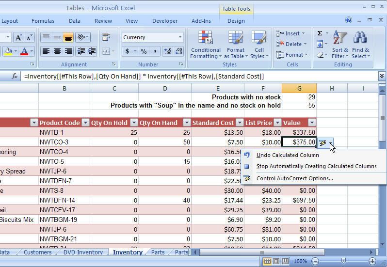
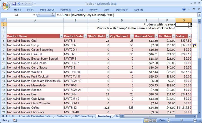
Cuối cùng, bạn cũng có thể tạo ra các dãy bằng cách sử dụng các tham chiếu có cấu trúc Table. Như với các tham chiếu ô thông thường, bạn tạo dãy bằng cách chèn một dấu hai chấm ) giữa hai specifier. Ví dụ, tham chiếu sau đây bao gồm tất cả các ô dữ liệu trong field Qty On Hold và field Qty On Hand của Table Inventory:

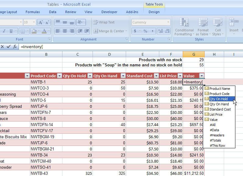
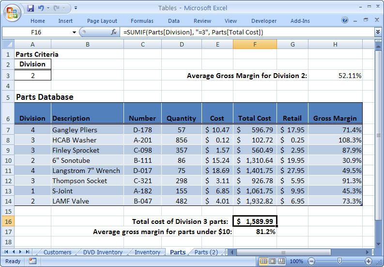
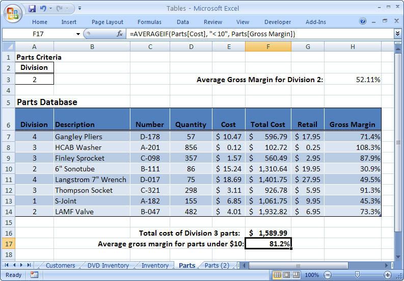
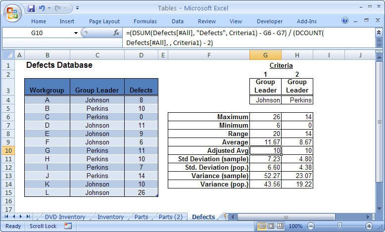
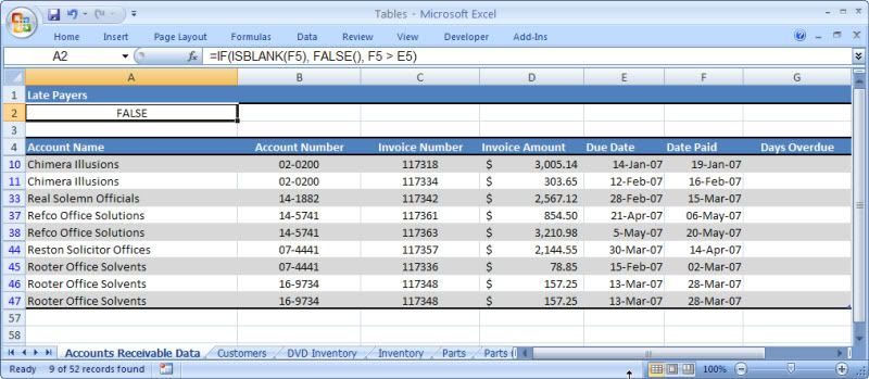
Inventory[[Qty On Hold]:[Qty On Hand]]​

 

[BNTT]

13.5. Sorting on Part of a Field


13.5.2. Entering Table Formulas
Nhập các công thức Table

When you build a formula using structured referencing, Excel offers several tools that make it easy and accurate. First, note that table names are part of Excel 2007’s new Formula AutoComplete feature. This means that after you type the first few letters of the table name, you’ll see the table name in the AutoComplete list, so you can then select the name and press Tab to add it to your formula. When you then type the opening square bracket ([), Excel displays a list of the table’s available specifiers, as shown in Figure 13.17. The first few items are the field names, and the bottom five are the built-in specifiers. Select the specifier and press Tab to add it to your formula. Each time you type an opening square bracket, Excel displays the specifier list.
Khi bạn xây dựng các công thức sử dụng loại tham chiếu có cấu trúc Table, Excel cung cấp một vài công cụ để làm cho nó dễ dàng và chính xác hơn. Đầu tiên, bạn hãy nhớ rằng các tên Table là môt phần của tính năng AutoComplete của Excel 2007. Có nghĩa là sau khi bạn gõ một vài ký tự đầu tiên của một tên Table, bạn sẽ thấy cái tên này trong danh sách AutoComplete, và bạn chỉ cần chọn nó, rồi nhấn phím Tab để thêm nó vào trong công thức của mình. Khi bạn gõ thêm một dấu ngoặc vuông mở ([), Excel sẽ hiển thị một danh sách các specifier có trong Table, như minh họa ở hình 13.17. Trong hình này, vài mục đầu tiên là các tên field, còn những cái ở dưới là các specifier có sẵn. Bạn chọn một specifier và nhấn Tab để thêm nó vào trong công thức. Mỗi lần bạn mở một dấu ngoặc vuông ([), Excel lại hiển thị danh sách các specifier.

Figure 13.17 - Tables.xlsx​

One of my favorite new features in Excel 2007 is its support for automatic calculated columns. To see how this works, Figure 13.18 shows a completed formula that I’ve typed into a table cell, but haven’t yet completed. When I press Enter, Excel automatically fills the same formula down into the rest of the table’s rows, as you can see in Figure 13.19. Excel also displays an AutoCorrect Options smart tag that enables you to reverse the calculate column, if desired.
Một trong những tính năng mới của Excel 2007 là nó hỗ trợ viêc tự động tính toán các cột (trong Table). Để thấy nó làm việc như thế nào, hình 13.18 minh họa một công thức hoàn chỉnh mà tôi đã gõ vào trong một ô của Table, nhưng chưa hoàn tất (chưa nhấn Enter). Khi tôi nhấn Enter, Excel tự động điền các công thức tương tự xuống các hàng còn lại trong cột đó, như bạn thấy trong hình 13.19. Excel cũng hiển thị một dấu hiệu AutoCorrect Options để cho phép bạn đảo ngược lại việc tính toán, nếu muốn.

Figure 13.18

Figure 13.19 - Tables.xlsx​

 

[BNTT]

Chapter 13 - Analyzing Data with Tables


13.6. Excel’s Table Functions
Các hàm Table của Excel

To take your table analysis to a higher level, you can use Excel’s table functions, which give you the following advantages:
Để làm cho việc phân tích các Table của bạn có một tầm cao hơn, bạn có thể sử dụng các hàm (thường hay sử dụng với các) Table của Excel, các hàm này có những ưu điểm sau:

• You can enter the functions into any cell in the worksheet.
  Bạn có thể nhập các hàm này vào bất kỳ ô nào trong bảng tính.
  
  
• You can specify the range the function uses to perform its calculations.
  Bạn có thể chỉ định dãy mà hàm sử dụng để thực hiện việc tính toán.
  
  
• You can enter criteria or reference a criteria range to perform calculations on subsets of the table.
  Bạn có thể nhập tiêu chuẩn (điều kiện) hoặc tham chiếu đến một dãy tiêu chuẩn để thực hiện các phép tính trên một phần nhỏ của Table.