- Tham gia
- 3/7/07
- Bài viết
- 4,946
- Được thích
- 23,213
- Nghề nghiệp
- Dạy đàn piano
Phỏng dịch từ cuốn Formulas and Functions with Microsoft Office Excel 2007 của Paul McFedries
Part I: MASTERING EXCEL RANGES AND FORMULAS - Nắm vững các dãy và công thức trong Excel
Chapter 5 - TROUBLESHOOTING FORMULAS
Xử lý các lỗi của công thức
IN THIS CHAPTER:
Những nội dung chính trong chương này:
Part I: MASTERING EXCEL RANGES AND FORMULAS - Nắm vững các dãy và công thức trong Excel
- Chapter 1: Getting The Most Out Of Range - Tận dụng tối đa các dãy
- Chapter 2: Using a Range Name - Sử dụng tên cho dãy
- Chapter 3: Building Basic Formulas - Thiết lập các công thức (cơ bản)
- Chapter 4: Creating Advanced Formulas - Thiết lập các công thức (nâng cao)
- Chapter 5: Troubleshooting Formulas - Xử lý lỗi công thức
Chapter 5 - TROUBLESHOOTING FORMULAS
Xử lý các lỗi của công thức
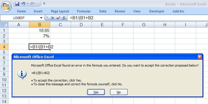
Despite your best efforts, the odd error might appear in your formulas from time to time. These errors can be mathematical (for example, dividing by zero), or Excel might simply be incapable of interpreting the formula. In the latter case, problems can be caught while you’re entering the formula. For example, if you try to enter a formula that has unbalanced parentheses, Excel won’t accept the entry; it displays an error message instead. Other errors are more insidious. For example, your formula might appear to be working — that is, it returns a value — but the result is incorrect because
the data is flawed or because your formula has referenced the wrong cell or range.
Cho dù bạn có cố gắng đến cỡ nào, thì thỉnh thoảng vẫn có những cái lỗi kỳ lạ xuất hiện trong công thức của bạn. Những lỗi này có thể là về toán học (ví dụ, chia cho không), hoặc Excel dường như không hiểu được các công thức. Trong trường hợp thứ hai này, các lỗi có thể sẽ được bắt gặp trong khi bạn gõ công thức. Ví dụ, nếu bạn cố nhập một công thức có các dấu ngoặc đơn không cân bằng (thiếu hoặc thừa dấu mở hoặc đóng ngoặc), Excel sẽ không chấp nhận công thức, thay vào đó, nó hiển thị một thông báo lỗi. Những lỗi khác mang tính ngấm ngầm hơn. Ví dụ, công thức của bạn có vẻ như vẫn làm việc — nghĩa là nó trả về một giá trị — nhưng kết quả thì sai, bởi vì dữ liệu bị sai sót hoặc bởi vì công thức tham chiếu đến ô hay dãy không đúng.
Whatever the error and whatever the cause, formula woes need to be worked out. But don’t fall into the trap of thinking that your spreadsheets are problem free. And the more complex the model is, the greater the chance is that errors can creep in. A KPMG study from a few years ago found that a staggering 90% of spreadsheets used for tax calculations contained errors.
Cho dù lỗi là gì và nguyên nhân là gì, những điều phiền toái của công thức cũng phải được giải quyết. Nhưng đừng bao giờ nghĩ rằng các bảng tính của bạn không có lỗi. Và một mô hình (một bảng tính do bạn phác thảo ra) càng phức tạp, thì khả năng các lỗi có thể xảy ra càng nhiều.
The good news is that fixing formula flaws need not be drudgery. With a bit of know-how and Excel’s top-notch troubleshooting tools, sniffing out and repairing model maladies isn’t hard. This chapter tells you everything you need to know.
Việc sửa các lỗi công thức không phải là một công việc khó nhọc. Với một chút hiểu biết và những công cụ xử lý sự cố hàng đầu của Excel, việc tìm ra và xử lý các chứng bệnh (của mô hình) thì không khó lắm. Chương này sẽ cho bạn mọi thứ mà bạn cần biết.
IN THIS CHAPTER:
Những nội dung chính trong chương này:
- Understanding Excel’s Error Values
Tìm hiểu về các Giá Trị Lỗi trong Excel
- Fixing Other Formula Errors
Sửa các lỗi công thức khác
- Handling Formula Errors with IFERROR()
Xử lý các lỗi công thức bằng Hàm IFERROR()
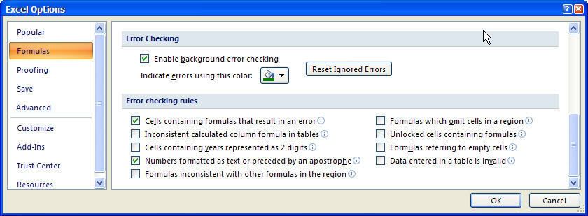
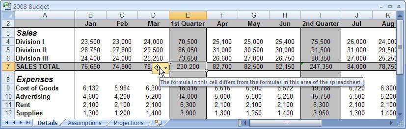
- Using the Formula Error Checker
Sử dụng công cụ kiểm tra lỗi công thức (Formula Error Checker)
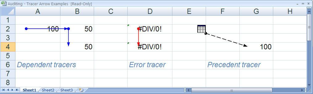
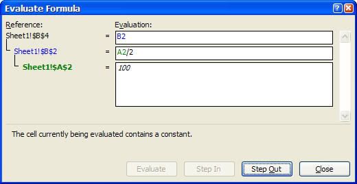
- Auditing a Worksheet
Kiểm tra một bảng tính
Lần chỉnh sửa cuối:
 ).
). 4 have no common cells, so the following formula returns the #NULL! error: